How we made AWS Trainium 17x faster (for conv1d)
November 17, 2025
Huijae An and Charles Hong
UC Berkeley
In this post, we take a deeper look at how Autocomp optimizes the conv1d_depthwise_default kernel provided by the AWS Neuron Team, achieving a 17.37x speedup in the final implementation.
📋 Table of Contents
About conv1d
1D convolution (conv1d) is a specialized case of a standard 2D convolution where the filter height is fixed to 1. If you’re familiar with conv2d, you can think of conv1d as sliding a narrow filter horizontally across a single spatial dimension.
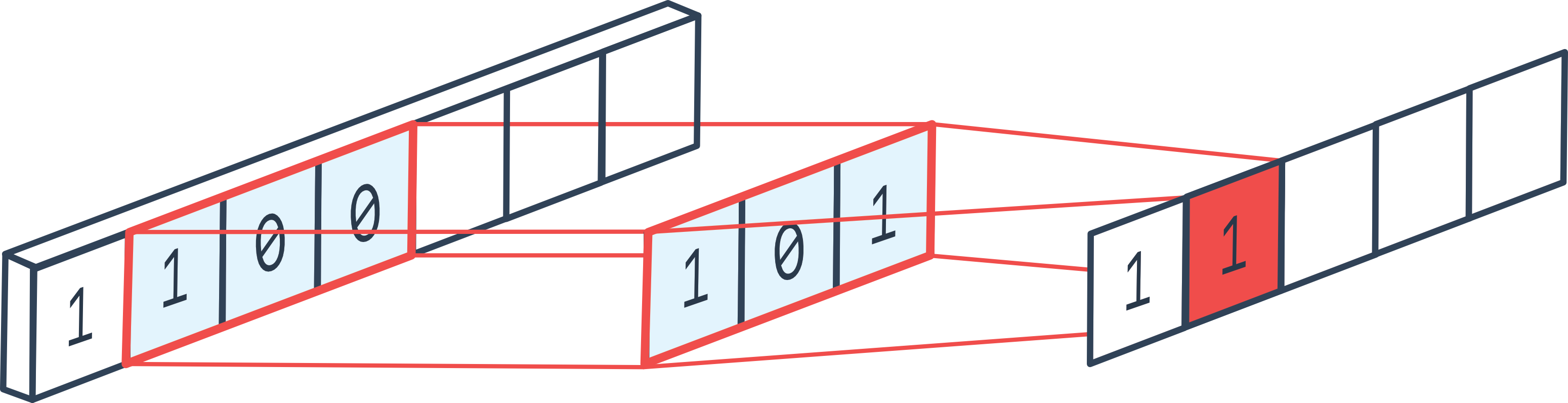
In our case, the kernel performs a depthwise 1D convolution, meaning each input channel is convolved independently with its own filter (meaning in_channel = out_channel).
Here’s the rough pseudocode of the original kernel:
def conv1d_depthwise_default(img, filters, output):
    """
    Input Shape: [N, C_in, 1, W]
    Filter Shape: [C_out, 1, 1, W_f]
    Output Shape: [N, C_out, 1, W]
    """

    # 1. Fetch the input into Trainium's Scratchpad (SBUF)
    img_local_prefetch_raw = nl.array(...)
    for n in range(N):
        for c_tiled in range(C_in // 128):
            img_local_prefetch_raw[n, [c_tiled+:128], :, :] = nl.load(...)

    # 2. Fetch the filters into Trainium's Scratchpad (SBUF)
    filter_local = nl.array(...)
    for c_tiled in range(C_out // 128):
        filter_local[[c_tiled+:128], :, :, :] = nl.load(...)

    # 3. Allocate the temporary output in Trainium's Scratchpad (SBUF)
    out_sb = nl.array(...)

    # 4. Perform depthwise convolution
    for n in range(N):
        for c_tiled in range(C_in // 128):
            for w in range(W):
                prod = nl.multiply(img_local_prefetch_raw[n, [c_tiled+:128], :, [w+:W_f]], filter_local[[c_tiled+:128], :, :, :])
                out_sb[n, [c_tiled+:128], :, w] = nl.sum(prod)

    # 5. Write the results back to the output in HBM
    for n in range(N):
        for c_tiled in range(C_out // 128):
            nl.store(output[...], out_sb[...])
Note that the output width matches the input width, rather than input_width − filter_width + 1. This is because we apply zero-padding on both sides of the input so that the output size stays consistent with the input.
In this case, we use N = 8, in_channel = out_channel = 512, image_width = 2048, and filter_width = 3 . Part of Autocomp’s speedup comes from taking advantage of optimizations specific to this shape.
Lastly, to take advantage of Trainium’s optimized execution on 128-channel groups, we tile in_channel (and out_channel, since they’re the same) into groups of 128. This layout is key to achieving high performance, and as we go through the optimization steps, we’ll see how Autocomp gradually leverages this structure to push the kernel closer to Trainium’s full potential.
Optimization Steps
Step 0
We first begin by pre-processing the kernel to make it easier to pass into Autocomp. Aside from stylistic changes and inlining helper functions that were previously declared outside the kernel, the only notable functional change is that we explicitly allocate and return the output tensor inside the kernel, instead of accepting a reference and modifying it in-place. This is necessary to comply with NKI compiler requirements and run the kernel standalone.
Pseudocode
def optimize_0(img, filters):
    # Inlined helper functions
    def div_ceil():
    def create_indices():

    # Explicitly allocate the output tensor in HBM instead of taking it as an argument
    out_hbm = nl.array(...)

    # ... (same as before)

    return out_hbm
Slowest nc_latency from 10 samples (with 2 warmup iters): 8.007 ms
Step 1
Autocomp attempts a hoisting optimization where it moves indexing of the loop-invariant filter_local[c_tile, i_p_a, i_f_a] tile outside of the innermost convolution loop, and assigns it to a new variable filt_tile. However, as we are indexing into SBUF, indexing is a logical operation that does not actually increase computation or data movement. As a result, latency remains the same.
Pseudocode
def optimize_1(img, filters):
    # ... (same as before)

    # 4. Perform depthwise convolution
    for n in range(N):
        for c_tiled in range(C_in // 128):
            # HOISTED: reuse the same filter sub-tile for all w
            filt_tile = filter_local[[c_tiled+:128], :, :, :]
            for w in range(W):
                prod = nl.multiply(img_local_prefetch_raw[n, [c_tiled+:128], :, [w+:W_f]], filt_tile)
                out_sb[n, [c_tiled+:128], :, w] = nl.sum(prod)

    # ... (same as before)
Latency: 8.007 ms (same as baseline)
Step 2
The kernel uses the helper function create_indices to generate broadcastable arrays for mapping indices (analogous to NumPy’s ogrid). One location where create_indices is used is at the end of the kernel, when writing results back to HBM. Autocomp removes create_indices in an attempt to “aggregate stores” and reduce the number of emitted store instructions, but the transformed code is semantically identical to the original. As a result, store behavior is unchanged and the latency remains essentially the same.
Note that in the first 2 optimization iterations, we allow slight increases in latency in order to encourage exploration in the initial stages of search.
[Pseudocode omitted]
Latency: 8.010 ms (0.99x speedup)
Step 3
Autocomp starts to make noticeable improvements to the kernel. It begins so by “optimiz[ing] memory buffer allocation” in the form of several optimizations:
- Fetching only the required portions of the input and filter within each loop iteration, instead of prefetching the entire tensors into SBUF before entering the loop. This helps with reducing the SBUF pressure.
- Replacing
nl.loadwithnisa.dma_copy, though they’re semantically the same. - Removing the use of
create_indicesentirely by generating a reusable tile, similar to step 2. - Fusing loops with identical boundaries, allowing for more aggressive compiler optimizations per iteration.
- Allocating only the portion of the output currently being written in SBUF, then immediately writing it back to HBM, instead of storing the entire output in SBUF first and transferring it all at once.
Pseudocode
def optimize_3(img, filters):
    # Fuse everything into a single global loop
    out_hbm = nl.array(...)

    for n in range(N):
        for c_tiled in range(C_in // 128):
            # Allocate and fetch only the required portion per iteration to reduce SBUF pressure
            img_tile = nl.array(...)
            filt_tile = nl.array(...)
            out_tile = nl.array(...)

            # Replace nl.load with nisa.dma_copy (no effect)
            nisa.dma_copy(img_tile, img[n, [c_tiled+:128], :, :])
            nisa.dma_copy(filt_tile, filters[[c_tiled+:128], :, :, :])

            for w in range(W):
                # Omitted in pseudocode; no longer relies on create_indices
                prod = nl.multiply(img_tile[:, :, :, [w+:W_f]], filt_tile)
                out_tile[:, :, :, w] = nl.sum(prod)

            # Write to HBM immediately once results are ready
            nl.store(out_hbm[n, [c_tiled+:128], :, :], out_tile)

    return out_hbm
Latency: 7.934 ms (1.01x)
Step 4
Autocomp leverages PSUM to reduce memory traffic: for each convolution, instead of storing every output element directly to SBUF, it first stores them in PSUM, then performs a single PSUM → SBUF transfer using nisa.tensor_copy. To ensure this PSUM buffer does not exceed its free-dimension limit, the kernel divides the convolution into blocks of size
F_BLK = min(out_image_size, nl.tile_size.psum_fmax).
Pseudocode
def optimize_4(img, filters):
    # ... (same as before)

            # Group W into batches of 512
            F_BLK = min(W, nl.tile_size.psum_fmax) # nl.tile_size.psum_fmax = 512
            for w_tiled in range(W // F_BLK):
                out_psum = nl.array(...) # shape: [128, F_BLK]
                blk_base = F_BLK * w_tiled # starting index within W
                # Convolve, then write to the corresponding free dimension of PSUM
                for f in range(F_BLK):
                    prod = nl.multiply(img_tile[:, :, :, [blk_base+:W_f]], filt_tile)
                    out_psum += nl.sum(prod)
                # Copy PSUM data into SBUF
                out_sbuf_blk = nisa.tensor_copy(out_psum)
                # Write the copied portion to HBM
                nl.store(out_hbm[n, [c_tiled+:128], :, blk_base+:F_BLK], out_sbuf_blk)

    return out_hbm
Profiling Results
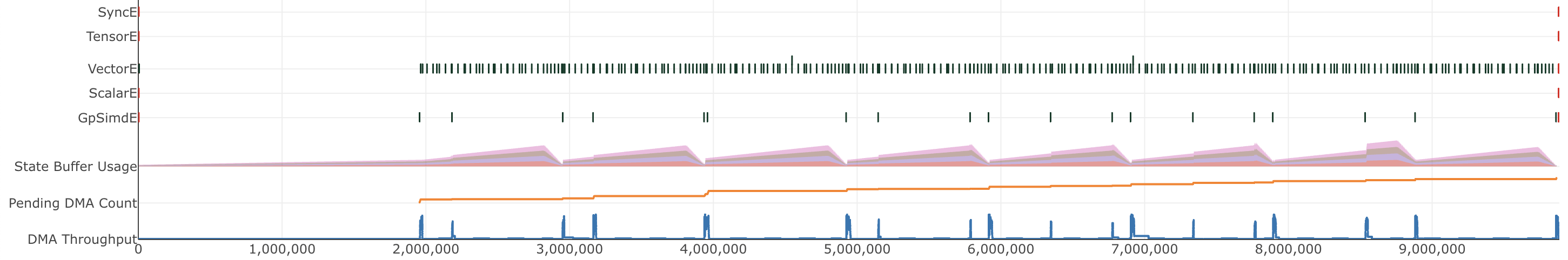
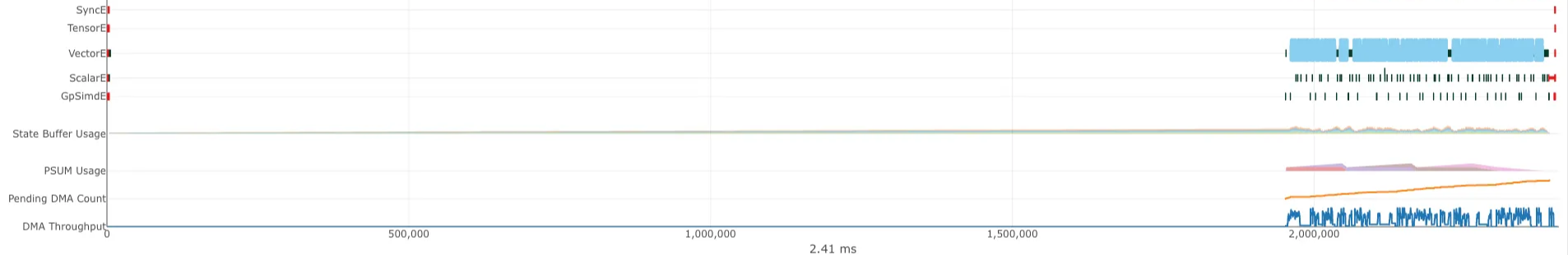
Now, let’s use Trainium’s neuron_profile tool to take a deeper look at the differences before and after this optimization. Here is what the profile viewer shows us before the Step 4 optimization (i.e., optimize_3):
And after (optimize_4):
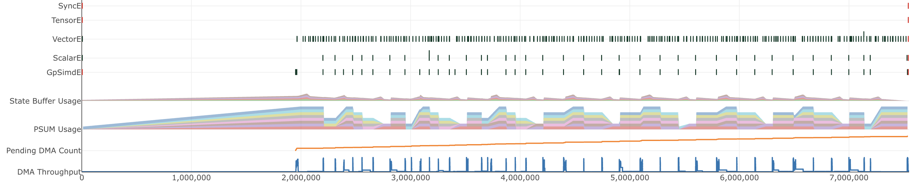
We see that once PSUM is utilized, the pressure on SBUF decreases and access to the filter weights becomes faster, leading to greater overall throughput and decreasing latency.
Latency: 5.602 ms (1.43x)
Step 5
Autocomp reuses the loaded filter weights by swapping the loop order: it swaps the loop order from “for each image → for each input channel” to “for each input channel → for each image”, allowing the same filter weights to be reused across multiple images.
At the same time, Autocomp discards the Step 4 optimization that used PSUM to accelerate nl.multiply operations; it chooses to store the reusable filter weights in PSUM instead. Because PSUM has limited capacity and we want to avoid fill-and-reloads, Autocomp prioritizes placing the filters there. We see that this strategy results in a greater speedup than the previous optimization.
Pseudocode
def optimize_5(img, filters):
    out_hbm = nl.array(...)

    # Reorder the most & second most outer loops
    for c_tiled in range(C_in // 128):
        # Fetch the reusable filter and store in PSUM
        filt_sbuf = nl.load(filters[[c_tiled+:128], :, :, :])
        filt_psum = nisa.tensor_copy(filt_sbuf)
        for n in range(N):
            img_tile = nl.load(img[n, [c_tiled+:128], :, :])
            out_tile = nl.array(...)

            for w in range(W):
                prod = nl.multiply(img_tile[:, :, :, [w+:W_f]], filt_psum)
                out_tile[:, :, :, w] = nl.sum(prod)

            nl.store(out_hbm[n, [c_tiled+:128], :, :], out_tile)

    return out_hbm
Latency: 4.955 ms (1.62x)
Step 6
Inside the convolution loop, Autocomp tiles the output width dimension into groups of 64.
for w in range(W):for w_out_tile in range(W // 64):
for w_in_tile in range(64):
w = w_out_tile * 64 + w_in_tileWhat’s interesting here is that the transformation is syntactic - the kernel does not actually process each 64 element group as a single combined operation; i.e., there is no manual coalescing of nl.multiply (actually implemented as tensor_tensor) or nl.sum (actually implemented as tensor_reduce) operations into a smaller number of larger operations in the code. However, this restructuring is enough to signal to the compiler that the work can be grouped, enabling it to aggressively schedule and optimize the convolution as if those 64 outputs were actually being processed together.
It isn’t entirely clear why Autocomp chooses a tile size of 64 instead of the more intuitive 128. However, we find that regardless of the value chosen, tiling by values near 128 (such as 32 or 64) appears enough for the compiler to perform its own grouping by a factor of 128, as we see from the operation counts we show below.
Pseudocode
def optimize_6(img, filters):
    # ... (same as before)

            NUM_FULL_BLOCKS = W // 64
            for w_out_tile in range(NUM_FULL_BLOCKS):
                base_out = w_out_tile * 64
                for w_in_tile in range(64):
                    prod = nl.multiply(img_tile[:, :, :, [(base_out + w_in_tile)+:W_f]], filt_psum)
                    out_tile[:, :, :, base_out + w_in_tile] = nl.sum(prod)
            nl.store(out_hbm[n, [c_tiled+:128], :, :], out_tile)

    return out_hbm
Profiling Results
For context, here is what the profile viewer shows us before the Step 6 optimization (optimize_5):
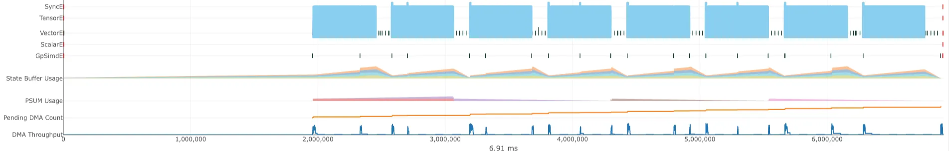
And after the optimization (optimize_6):
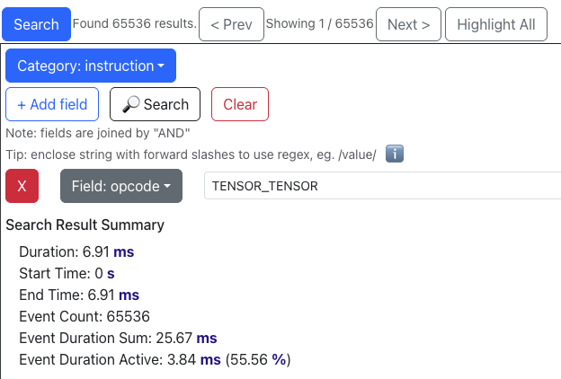
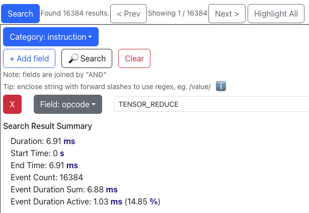
Before: In optimize_5, we had N * (C_in / 128) * W = 65536 individual tensor_tensor operations. We also had 65536 / 4 = 16384 individual tensor_reduce operations. This seems to imply that the NKI compiler is eagerly fusing tensor_reduce calls across four partition tiles at a time when the total number of tensor_reduce calls in a loop is unknown at compile time. If any Trainium experts can confirm this, please let us know!
These instructions combined were active for about 70% (55.56% + 14.85%) of the total profiled time, making them a prime target for optimization according to Amdahl’s law.
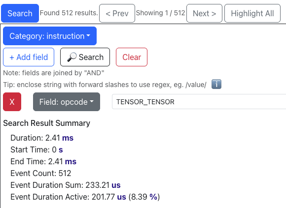
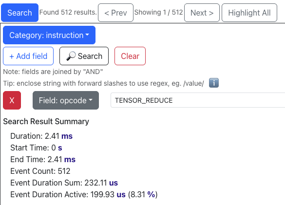
After: In optimize_6, we see that the number of tensor_tensor and tensor_reduce operations are now both just 512 (equal to 65536 / 128), meaning both operations are now likely being fused across 128 partition tiles. Their execution times decrease from 3.84 → 0.2ms and 1.03 → 0.2ms, now totaling only 17% (8.39% + 8.31%) of the profiled runtime. Since the kernel is primarily compute-bound on these two operations, this reduction leads to a substantial overall speedup.
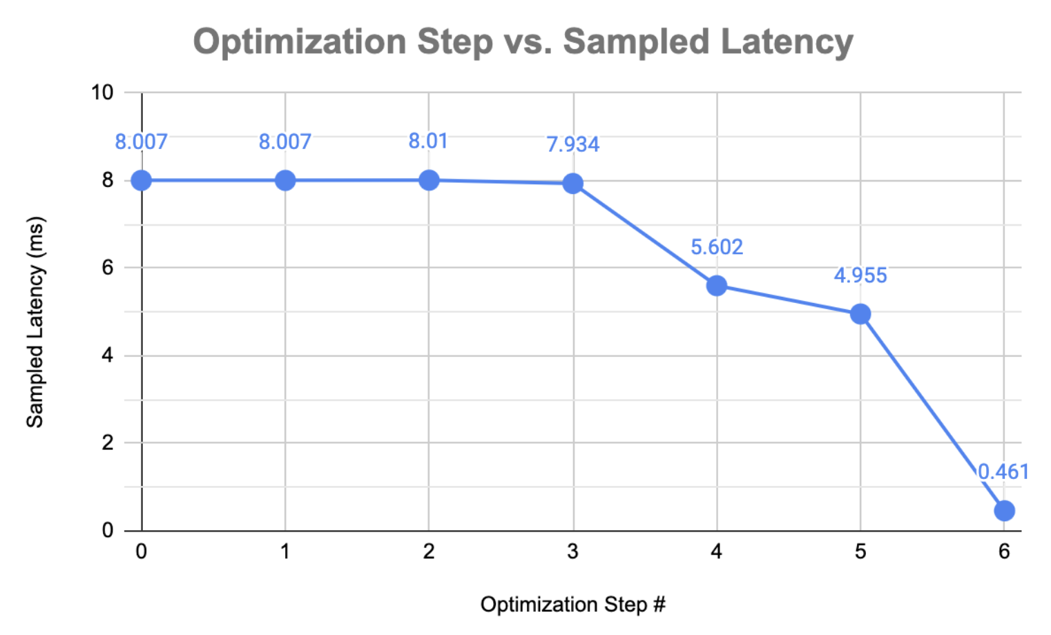
Latency: 0.461 ms (17.37x)
Conclusion
Speedup Summary:
| Optimization | Latency (ms) | Speedup |
|---|---|---|
| Baseline | 8.007 | 1.00x |
| Hoisted Filter Indexing | 8.007 | 1.00x |
Removed create_indices |
8.010 | 0.99x |
| Loop Fusion + Optimized Memory Buffer Allocation | 7.934 | 1.01x |
| PSUM Buffer Allocation | 5.602 | 1.43x |
| Loop Order Interchange | 4.955 | 1.62x |
| Tile Hint | 0.461 | 17.37x |
In this case study, we saw how Autocomp applies a range of kernel optimization techniques to improve the conv1d kernel provided by the AWS Neuron team. From conventional memory traffic optimizations to NKI-specific behaviors, Autocomp systematically transformed the code, exploring design spaces and edge cases that human kernel writers might not easily consider. We’re excited to continue expanding our use of Autocomp and see what other applications it can optimize next.
Thanks to Huijae An, a talented undergrad researcher working with us in the SLICE Lab, for leading the writeup of this blog post, and Haozheng Fan from the Neuron Science team for providing feedback and insights.